AffineGS: Unlocking Accurate Geometry in 3DGS via Spatially Varying Affine Rectification

Tze Ho Elden Tse^1,2*

Jizong Peng^1*

Richard Chen¹

Angela Yao²

¹dConstruct Robotics, ²National University of Singapore ^*Equal contribution NeurIPS 2026

[Paper]

[GitHub]

TL;DR: Monocular depth priors are distorted piecewise-linearly, not globally. We rectify them with spatially varying, edge-aware affine fields, which gives 3DGS accurate geometry without sensor-depth supervision.

0.71 vs 0.28

Mesh F-score on MuSHRoom vs. DN-Splatter using the same monocular prior

6× lower

Depth error on MuSHRoom
(Abs Rel 0.055 vs. 0.354)

up to +4 dB

PSNR over the best baseline in sparse-view (2–5 views) NeRF-LLFF

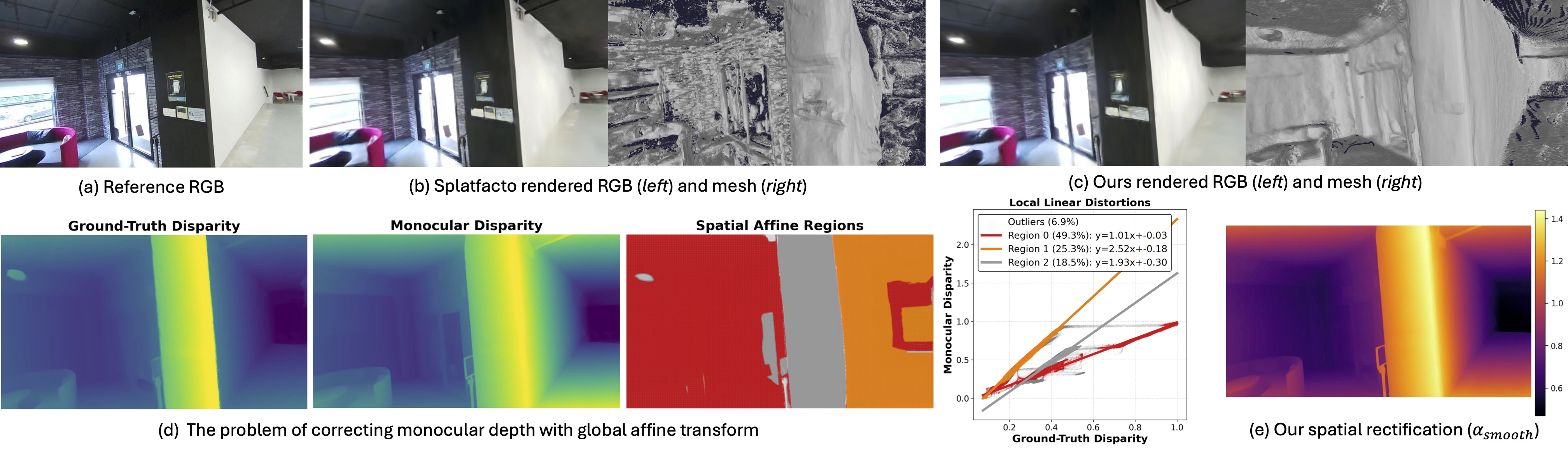
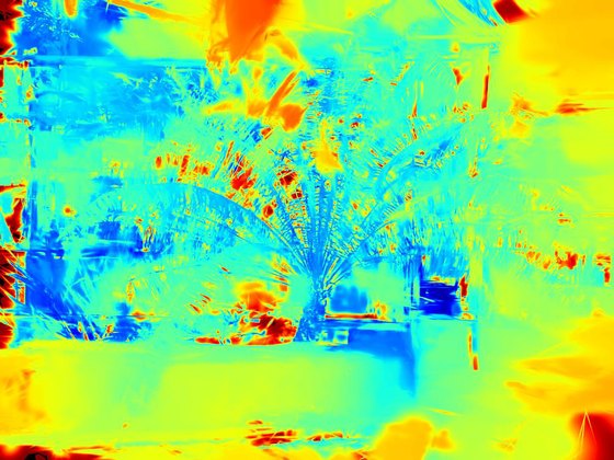
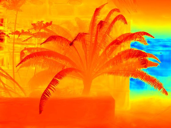
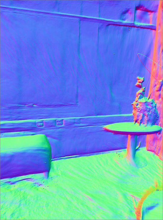
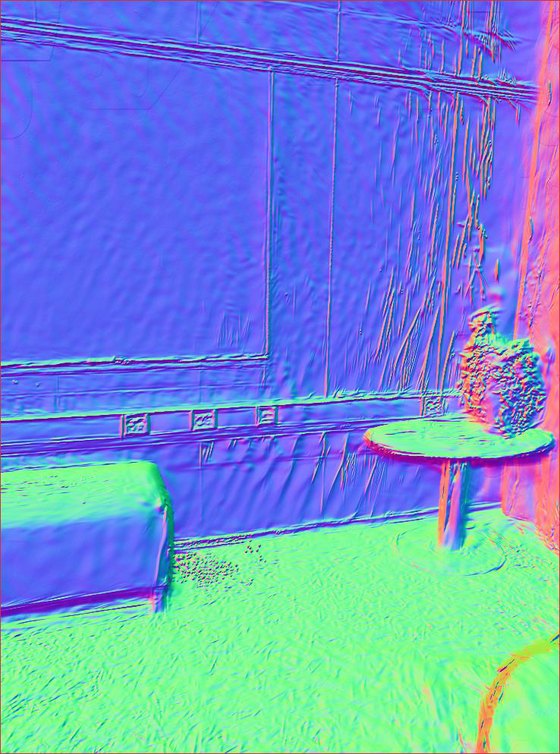
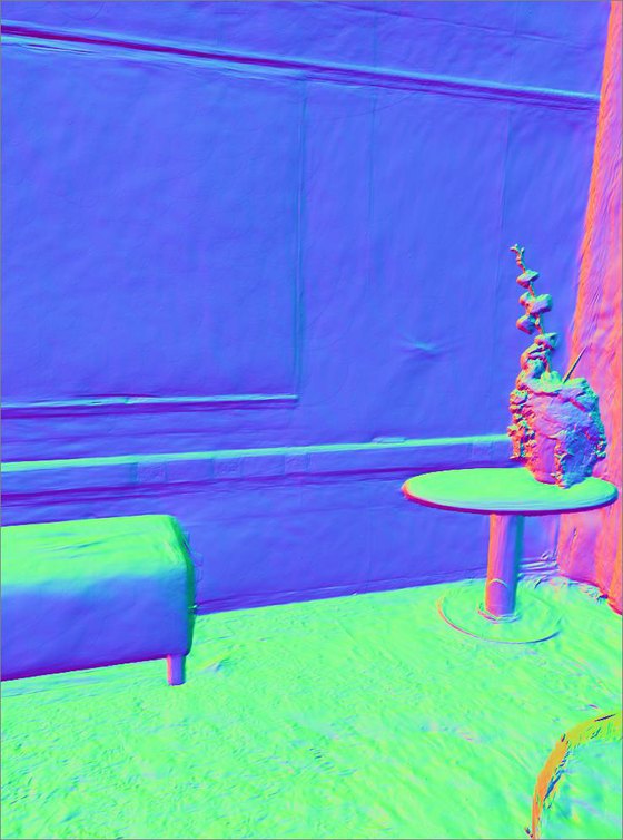
(a-c) Standard 3DGS overfits appearance, producing noisy underlying geometry. In contrast, our method extracts clean, highly accurate meshes while maintaining photorealism. (d) Monocular disparity exhibits piecewise-linear distortions, proving that a single global scale-and-shift alignment is fundamentally insufficient (scatter plot). (e) We overcome this by estimating an edge-aware spatial scale field to rectify the monocular depth prior, yielding geometrically consistent 3D representations.

Abstract

3D Gaussian Splatting (3DGS) has become the leading approach for photorealistic novel view synthesis, yet its underlying geometric accuracy lags behind its visual quality. Existing depth-guided methods attempt to resolve this by regularizing the optimization with monocular depth priors, typically relying on a global linear alignment. Crucially, we reveal a fundamental flaw in this assumption: modern monocular depth networks systematically exhibit region-dependent, piecewise-linear distortions. This phenomenon invalidates standard global alignment strategies, which inevitably warp scene geometry by enforcing a single scale-and-shift transform. To address this, we introduce a spatially varying affine rectification model that dynamically corrects monocular disparity into consistent metric depth using regionally smooth, edge-aware fields. We further derive a normal-aware regularizer that uses spatial gradients to couple the rectified disparity with 3DGS depth and normals. Extensive evaluations demonstrate that our sensor-free approach prevents structural collapse under extreme view sparsity and extracts highly accurate 3D meshes, effectively bridging the gap toward sensor-supervised geometric fidelity while preserving state-of-the-art photorealism.

Key Observation

Depth-guided 3DGS methods usually assume that monocular disparity can be aligned to metric depth with a single global scale-and-shift. We find that this assumption breaks down: modern monocular depth models (Depth-Anything-V2, MoGe, Metric3D-V2) show region-dependent, piecewise-linear distortions. The predicted disparity splits into distinct regions, with breaks along object boundaries and depth discontinuities, and each region follows its own linear relationship to the true depth.

Alignment Strategy	MuSHRoom		ScanNet++
Alignment Strategy	Inlier Ratio ↑	RMSE ↓	Inlier Ratio ↑	RMSE ↓
Global Affine (K = 1)	58.9%	0.074	58.6%	0.088
Piecewise Local (K = 3)	84.9%	0.046	84.6%	0.056
Piecewise Local (K = 5)	92.7%	0.030	91.8%	0.039

Depth-Anything-V2 prior, evaluated at a 0.02 residual threshold. A single global transform leaves over 40% of the scene misaligned. Splitting the image into just 3–5 local linear regions raises the inlier ratio above 84% and 91% and roughly halves the RMSE.

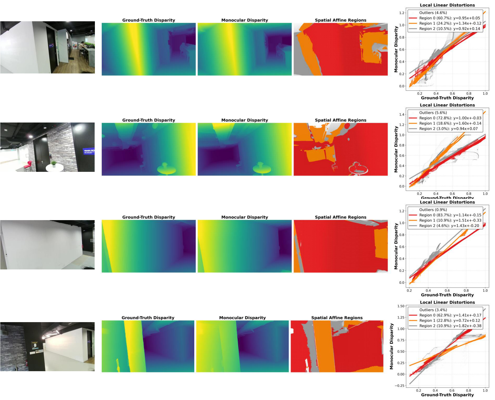
Across diverse indoor scenes, the monocular disparity consistently fractures into spatially coherent affine regimes (red, orange and grey). The scatter plots show that one global scale-and-shift (K = 1) cannot fit these incompatible linear clusters: it either averages the error across all of them or fits the dominant region and warps the rest. Our method instead estimates spatially varying, edge-aware affine fields that rectify each region locally.

Method

Instead of a single global scale-and-shift, we model the relationship between the monocular disparity d and the rendered 3DGS depth D as a spatially varying affine transform, 1/d(u,v) = α(u,v) D(u,v) + β(u,v). The fields are recovered without any sensor depth and re-estimated at every training iteration.

Rendering & monocular prior. 3DGS renders depth D and normals n for a training view, and a pre-trained Depth-Anything-V2 predicts its monocular disparity d.
Spatially varying affine rectification. Because the affine fields vary much more slowly than depth within coherent regions, the gradients satisfy −∇d/d² ≈ α∇D. We solve for the local scale α from the finite-difference gradient magnitudes, recover the shift β, and smooth both with an edge-aware guided filter that uses d as the guide. The fields stay smooth within surfaces and sharp across object boundaries, matching the piecewise-linear structure of the distortions.
Geometric supervision. The rectified fields drive three losses:
- Gradient loss: matches predicted and measured disparity gradients in magnitude and direction.
- Normal-aware loss: derives depth gradients from the rendered normals via pinhole projection, so the orientations of the Gaussians align with the scene's local slopes.
- Metric re-alignment loss: an L1 depth loss on the rectified depth that prevents global scale drift.

The method changes neither the Gaussian representation nor the densification. All gains come from the supervision signal.

Results

Sparse-view reconstruction (NeRF-LLFF)

With only 2–5 training views, our rectified prior prevents structural collapse and outperforms all baselines at every view count. It closes the gap to, and in some scenes surpasses, the Oracle, which uses dense multi-view pseudo-ground-truth depth.

Method	PSNR ↑				SSIM ↑				LPIPS ↓
Method	2	3	4	5	2	3	4	5	2	3	4	5
3DGS	13.31	15.13	17.37	18.68	.329	.437	.541	.601	.451	.348	.271	.226
DropGaussian	13.00	16.53	17.83	18.62	.386	.557	.622	.665	.444	.266	.229	.205
DepthSplat	13.98	16.68	17.97	18.32	.319	.391	.454	.472	.450	.383	.324	.334
DRGS	17.31	18.75	20.06	20.78	.475	.539	.601	.631	.324	.287	.249	.225
Ours	18.79	20.95	22.37	23.32	.533	.663	.721	.761	.235	.164	.134	.111
Oracle	19.88	21.76	22.83	23.93	.579	.670	.706	.746	.237	.177	.153	.129

Mean over the Fern, Flower, Fortress and Horns scenes and 10 random view selections; columns are the number of training views. Oracle (grey) is an upper bound that uses pseudo-ground-truth depth from all images.

Novel-view synthesis & depth (MuSHRoom)

Given the same Depth-Anything-V2 prior, globally aligned DN-Splatter (Monodepth) collapses structurally (Abs Rel 0.354). Our rectification cuts this to 0.055, compared with 0.023 for the sensor-supervised DN-Splatter, and matches DN-Splatter's photorealism.

Method	Sensor depth	PSNR ↑	SSIM ↑	LPIPS ↓	Abs Rel ↓	δ < 1.25 ↑
Splatfacto	–	24.44 / 21.33	.8486 / .7821	.1387 / .2240	.0787 / .0817	.9072 / .9061
2DGS	–	22.52 / 21.73	.8185 / .7898	.1773 / .1911	.0864 / .0923	.8820 / .8927
SuGaR	–	20.52 / 18.18	.7740 / .7125	.2427 / .2959	.1213 / .1174	.8412 / .8564
DN-Splatter (Monodepth)	–	19.26 / 17.24	.7255 / .6845	.3338 / .3851	.3542 / .3669	.5682 / .5818
Ours	–	24.49 / 22.07	.8570 / .7920	.1288 / .1733	.0551 / .0490	.9674 / .9729
DN-Splatter	✓	24.58 / 21.89	.8558 / .7984	.1293 / .1797	.0228 / .0354	.9854 / .9683

Explicit (Gaussian-based) methods, averaged over 6 scenes. Each cell shows the within-trajectory / disjoint-trajectory test split. Bold marks the best method without sensor depth. The sensor-supervised DN-Splatter (grey) is shown for reference.

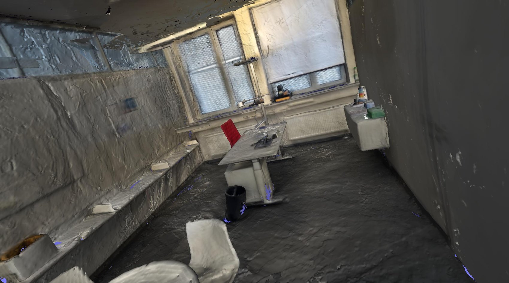
The globally aligned baseline warps the geometry. By rectifying the same monocular prior, our method recovers crisp planar surfaces and sharp object boundaries, better than DN-Splatter even with sensor depth.

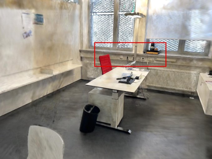
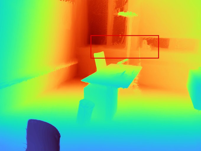
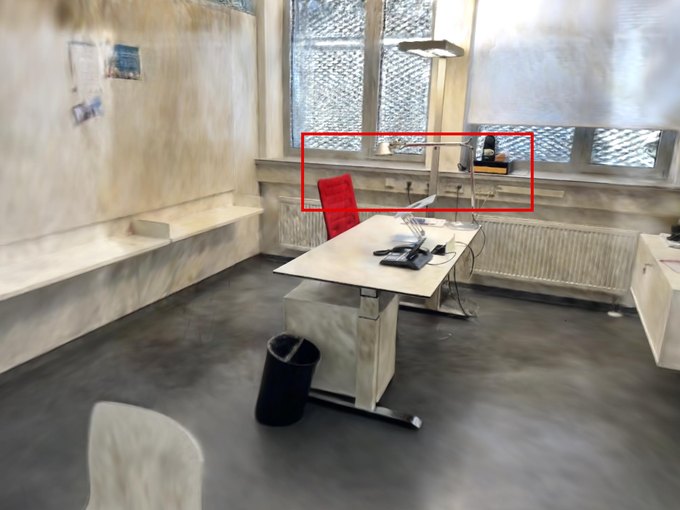
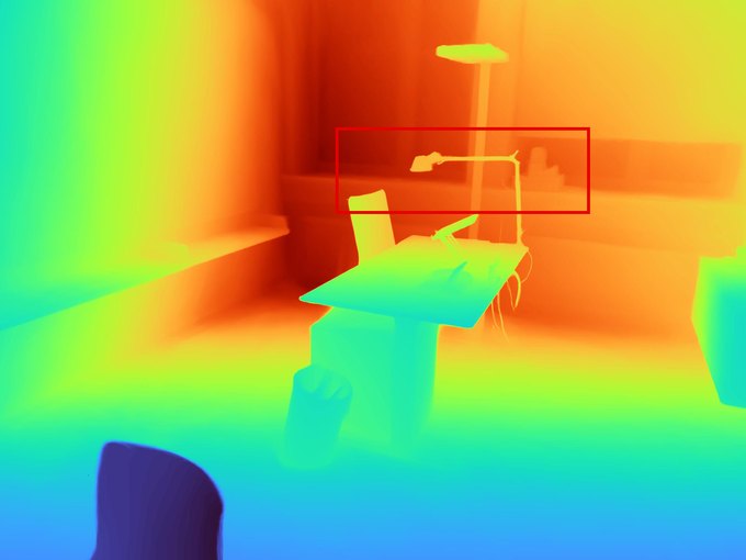
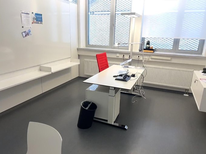
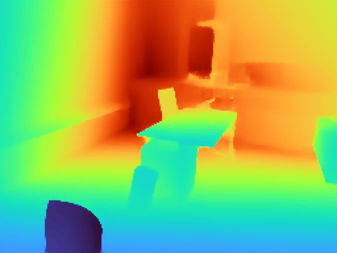
Rendered RGB (top) and depth (bottom) on ScanNet++. The red boxes highlight sharper depth along furniture boundaries and complex geometry.

Mesh reconstruction (MuSHRoom & ScanNet++)

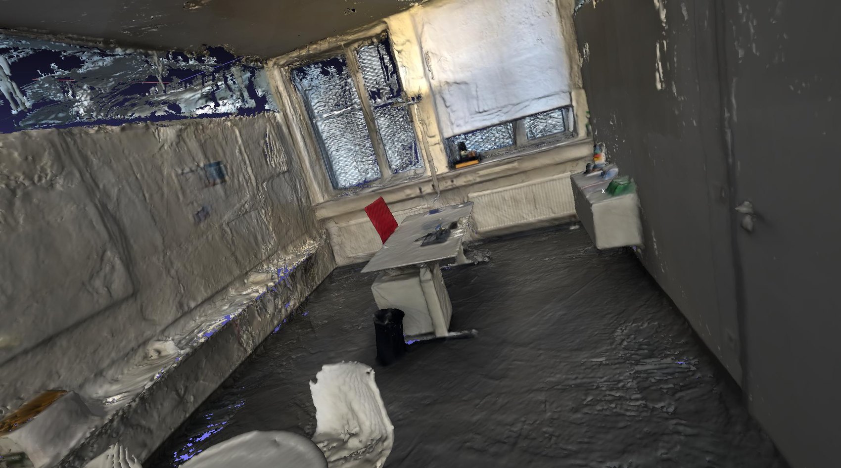
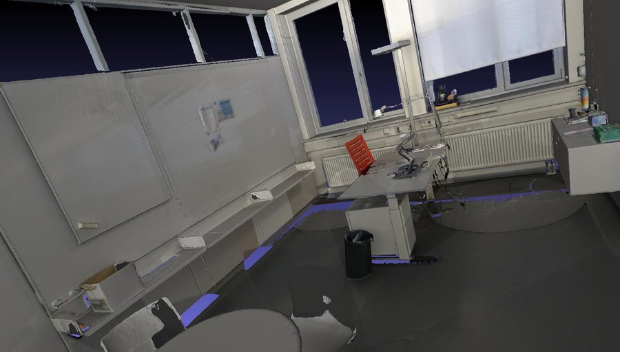
Without sensor depth, DN-Splatter's meshes degrade badly (F-score 0.28 on MuSHRoom). With the same monocular prior, our method reaches 0.71 and is the best sensor-free explicit method on both datasets, ahead of dedicated meshing methods such as SuGaR and 2DGS.

Method	Sensor depth	MuSHRoom			ScanNet++
Method	Sensor depth	Chamfer-L1 ↓	Normal C. ↑	F-score ↑	Chamfer-L1 ↓	Normal C. ↑	F-score ↑
Splatfacto	–	.0652	.7727	.5835	.1719	.6741	.1790
2DGS	–	.0687	.8008	.6039	.1035	.7799	.4196
SuGaR	–	.0620	.8031	.6378	.0975	.7241	.4367
DN-Splatter (Monodepth)	–	.2605	.6415	.2765	.1975	.7378	.1395
Ours	–	.0486	.8662	.7097	.0707	.8747	.4765
DN-Splatter	✓	.0216	.8822	.9243	.0667	.8316	.7658

Explicit methods; F-score at a 5 cm threshold. Bold marks the best method without sensor depth. The sensor-supervised DN-Splatter (grey) is shown as an upper bound.

DN-Splatter Ours

Drag the slider to compare extracted meshes on ScanNet++.

Ground-truth mesh. Our method also recovers the window geometry, which is missing from the ground truth.

Ablation

Each loss contributes to the result. L_depth anchors the global scale, L_normal keeps surfaces smooth, and L_grad ties disparity gradients to physical structure. Together, they trade a small PSNR drop for the best geometric accuracy.

Method	Photometry		Geometry
Method	PSNR ↑	LPIPS ↓	Abs Rel ↓	Accuracy ↓	F-score ↑
Splatfacto (baseline)	25.293	0.086	0.059	0.043	0.728
+ L_grad	24.322	0.123	0.085	0.054	0.673
+ L_normal	25.256	0.085	0.064	0.042	0.728
+ L_depth	24.561	0.098	0.043	0.030	0.798
+ L_grad + L_normal	24.553	0.116	0.075	0.051	0.707
+ L_grad + L_depth	25.012	0.101	0.041	0.026	0.850
+ L_normal + L_depth	25.418	0.084	0.040	0.028	0.813
All (Ours)	24.947	0.102	0.040	0.025	0.855

Evaluated on the coffee_room scene of MuSHRoom. Bold marks the best geometric results.

Paper and Supplementary Material

Tze Ho Elden Tse, Jizong Peng, Richard Chen, Angela Yao.
Unlocking Accurate Geometry in 3DGS via Spatially Varying Affine Rectification
NeurIPS, 2026
(hosted on ArXiv)

[Bibtex]

Acknowledgements

This template was originally made by Phillip Isola and Richard Zhang for a colorful ECCV project; the code can be found here.